1 INTRODUCTION
With the increasingly competitive business
environment, companies seek to improve their operations, so that profit is
optimized to reduce waste. To manage efficiently requires effective planning,
for this, it is necessary to have a perspective of the future conditions in
which the company will operate, and how the elements that condition this
perspective relate to each other [1].
To ensure competitive advantage, companies
rely on systems that allow them to expect how resources should be used. These
systems make it possible to extract information through large volumes of data
to provide insights. Thus, data mining helps in the extraction of information
from the database, being a great ally in planning corporate strategies, having
the ability to promote in managers a more adequate understanding of the current
situation of the company, thus allowing through insights the generation of
strategies to increase sales, as well as determining the direction to be
followed [2].
Sales is the core activity from a business process. Companies
record and document every transaction as a cycle in financial management. Sales
transaction data histories can be used to predict the possibility of sales
transactions that will occur in the future [3]. companies have invested
in decision support systems to explore scenarios based on the historical data
of their transactions.
Sales prediction is the
process of organizing and analyzing information in a way that makes it possible
to estimate how sales will be [2]. Thus, information technology is
transforming the way businesses are conducted. Data mining for sales prediction
is utilized for capturing the tradeoff between customer demand satisfaction and
inventory costs. An essential and inexpensive way for each company to augment
their profits, decrease their costs, and achieve greater flexibility to changes
[4].
1.1 OBJETIVES
The objective of this study
is to analyze the sales database to predict the number of sales. This research
uses a data mining-based approach for sales prediction. In this way, this study
proposes an improvement in financial management.
1.2 JUSTIFICATION
Currently,
sales transaction data histories are used to predict the possibility of sales
transactions that will occur in the future. However, this financial management
has no assertive predictability. Therefore, the identification of relevant
attributes and correlations for sales prediction becomes a fundamental factor
for competitive advantage. Decision-making systems help companies to augment their profits, decrease
their costs, and achieve greater flexibility to changes [4].
1.3 NEGATIVE SCOPE
It is not the objective of this study to generate a sales
prediction application or integration for the company's use, nor will we impose
the use of the metrics obtained or put them into practice to validate the
results obtained during the study.
2 THEORETICAL
FOUNDATIONS
2.1 DATA MINING
Decision making based on
experience and intuition alone is not always sufficient for solving complex
problems. One solution to this problem is the use of data mining algorithms to
assist in the decision-making process [5]. Data mining can be
understood as the process of analyzing large amounts of data in order to find
patterns, correlations, and anomalies to predict outcomes that, given the
volume of data, would not be easily discernible by human reason alone.
The data mining process
takes place in several steps, as a kind of filtering, so that in the end only
the information that really matters remains. The steps of this process can be
summarized in: 1) Business Understanding, 2) Data Selection, 3) Data Cleaning,
4) Data Modeling, 5) Process Evaluation, and 6) Execution. It is through these
steps that data mining surveys large volumes of data and relates them in a
useful way, thereby capturing the information relevant to the user's
objectives.
The general data mining
techniques can be summarized into five: Classification (consists of dividing
data into categories and the most commonly used algorithms for this purpose are
decision trees, regression and neural networks); Estimation (is estimation of a
probable value, compared to preexisting data and neural network and regression
algorithms can be used); Prediction (is the evaluation of a future data, taking
historical data and behavior as a parameter, and neural network, decision trees
and regression algorithms can be used); Cluster Analysis (aims to form groups
of elements that are more homogeneous among themselves, and is performed by
specific statistical algorithms, neural networks, and genetic algorithms), and
Affinity Analysis (seeks to recognize patterns of concomitant occurrence of
certain events in the analyzed data, using association rules most of the time) [6].
2.1.1 Algorithms
In this
research, some data mining algorithms were selected and will be described
below:
·
Linear Regression: model that considers the connection of responses to the
variable to be a linear function of some parameters, and this is done to ensure
generalization - giving the model the ability to predict outputs for inputs it
has never seen before.
·
Ridge CV: also known as L2, it’s a model fit method used to analyze any data that
suffers from multicollinearity. This technique discourages overfitting the data
in order to decrease its variance. As the L2 penalty is disproportionately
larger for larger coefficients, Ridge regularization causes correlated features
to have similar coefficients.
·
Support Vector Regression (SVR): supervised learning algorithm used to
predict discrete values that seeks to find a best-fit line. A
best-fit line is the hyperplane that has the maximum number of points. A big
benefit of using SVR is that it is a non-parametric technique.
·
LSTM: is a special kind of recurrent neural network (RNN), which
can remember information for much longer time periods and can capture complex,
nonlinear relationships due to its recurrent structure and gating mechanisms
that regulate the information flow into and out of the cell, and its large
capacity to deal with sequential data. Contrary to the classical neural
networks, LSTM has feedback connections that enable the processing of input
sequences of arbitrary length and is commonly preferred in classifying,
processing and making predictions based on time-series data [7]. It means that LSTM is a
good approach to use for sales forecasting. That is the reason why this was one
of the algorithms choosed.
·
ARIMA: is a combination of A.R. and M.A. models, along with
differencing. In Autoregressive models (A.R.), predictions are based on past
values of the time-series data, and in Moving Average models (MA), prior
residuals are considered for forecasting future values. The model is generally
favored for its flexibility to various types of time-series data and its
predicting accuracy [8]. For this reason, this was one of the
techniques selected to execute the sales forecasting.
2.1.2 Ensemble Methods
Ensemble
methods are a technique that use multiple learning algorithms and combine them
to achieve improved results on the predictive performance. Unlike other
techniques that will find a single model to make predictions for a specific
problem in a space with multiple hypotheses, ensembles will combine a - finite
- set of alternative models for that. This combination of multiple models
allows the elimination of variance, and because of that, increasing the
accuracy of predictions.
The
ensemble methods are divided into two categories: sequential ensemble
techniques, which generate base learners in a sequence; and parallel ensemble
techniques, which generate base learners in a parallel format. The first one
promotes dependence between the base learners, while the second one,
independence.
The
most popular ensemble methods are (i) boosting, (ii) bagging and (iii)
stacking. (i) Boosting is a technique that learns from mistakes made by the
previous predictor, in order to make better predictions. (ii) Bagging will
improve the results of the model through decision trees, reducing variance; and
(iii) Stacking, a technique that allows a training algorithm to ensemble other
similar learning algorithm predictions. The effectiveness of these methods,
throughout the years, has been proved undeniable, including in the improvement
of predictive models for sales forecasting [9].
2.2 SALES FORECASTING
Sales forecasting consists of the calculation or the sequence
of steps that the decision maker performs, based on a sales history and
understanding of the consumer, in order to predict the results of their sales.
The forecast gives insight into how a company should manage
its workforce, resources and cash flow, and also helps enterprise planning and decision-making
regarding operations, marketing, sales, production and finances in an effective
way. It also increases the commercial competitive advantage, as decision makers
will make the best choices using the information obtained through its
mechanism.
A sales
forecasting mechanism allows the organization to improve market growth with
greater revenue generation, and to create one with a high level of accuracy and
reliability is one of the biggest challenges. To achieve this, data mining
techniques are very effective in turning huge volumes of data into useful
information for sales forecasts [10].
2.2.1 Coupons Sale
Wholesale and retail
consumers normally, when making a purchase, get the change from their purchase
in return in bills and/or coins. The case study discussed here handles shopping
change differently. When buying a certain product in a store, the change
received by the customer will be provided as a complement through a virtual
coupon, which represents the change for a certain sale. In this way, the
customer will be getting his change in a virtual score format, being able to
compete for prizes, in which the higher the score, the greater are the chances
of winning. In this context, sales are represented by this additional change,
which can vary between R$0.10 and R$10.00.
2.2.2 Times Series Forecasting
A time series is a
collection of observations made sequentially over time. The order of the data is
a fundamental characteristic of this type of data since the dependency between
them is used for analysis and modeling [11]. Time series analysis
(TSA) refers to methods that analyze the characteristics of the data, to
extract useful statistics from them. Time series forecasting is often used to
predict future expected values of the data to be recorded. Time series analysis
has the undoubted advantage of being simple and effective, since the pertinent
outcomes can often be interpreted intuitively [12].
2.3 RELATED WORKS
As mentioned earlier, the company does not use its daily,
monthly, and yearly sales prediction based on the many variables that can
affect the sales quantity, such as store location, the day, month and time of
the sale, the value of the sales coupon, among others. This directly affects
the accuracy of the sales quantity in a given period, which can hinder
decision-making on various aspects of the company.
In this context, the study developed by Xiaodan, Yu, Zhiquan,
Qi, and Yuanmeng, Zhao, in 2013, proposes to use the sales forecast, but to
avoid excessive printing of magazines and newspapers, based on previous sales
data [10]. Thus, variables such as the type of store where the
newspapers and magazines are located, demographic data regarding the area where
the store is located, among others, are used. To perform predictability, the
SVR (Support Vector Regression) technique was used, which has the objective of
finding a function that matches the input data with the smallest possible error.
This method was used under the assertion that forecasting techniques such as
multiple regression and linear regression suffer from overfitting problems [13].
A study developed by Passari uses the approach of artificial
neural networks and their techniques to forecast retail sales. This work aims
to use ANNs to create individualized sales forecast models, that is, to analyze
each product individually [10]. Also, this research uses ANNs to
detect relationships among variables that impact the store sales volume (per
product), which is directly related to sales forecasting. Several other
techniques are mentioned, especially time series, but artificial neural
networks are the main focus.
Another research by Zadeh, Sepehri and Farvaresh applies
intelligent sales forecasts for drug distribution companies. In this specific
case, the sales forecasting mechanism proves to be quite effective as the
products of this industry quickly perish and the quality of these products
directly affects human health and life. The objective of this study was to
provide an accurate sales forecast model for auxiliary companies, especially
pharmaceutical companies, in order to predict the sale of products and avoid
costs caused by stock loss and customer loss due to lack of products. As a
main contribution a research, hybrid neural networks were carried out to let
linear ANN model the linear components and let nonlinear ANN model the
nonlinear components and then merge the results from both linear and nonlinear
models, as well as, adding a new method of product grouping that makes use of
past sale data in the prediction of sales and also helps gain more accuracy in
the predictions [4].
Another recent study
considered different machine-learning approaches for time series forecasting.
This research quotes regression approaches for sales prediction that gives
better results than time series methods. Their research provides improvement in
accuracy on the validation and on the out-of-sample data sets using an ensemble
method. The use of a stacking approach makes it possible to take into account
the differences in the results for multiple models with different sets of
parameters [9].
3 MATERIALS
AND METHODS
3.1 DATABASE DESCRIPTION
The database provided was exported from sales data from the
company points program, it has over 1.5 million entries and is composed of two
tables, the first being the sales table and the second a table with data from
the establishment where the sale was executed, where we filtered only the city
and the state.
Each entry in the sales table corresponds to a sale made at a
POS (point of sale), which in this case corresponds to one of the cash
registers of the several commercial establishments that are part of the
program.
For data privacy reasons,
the commercial establishments where the sales were made had their data
encrypted and are identified through an ID. In addition, the base is composed
of the value of the coupon purchased by the customer, the date and time of the
purchase, as well as the city and state in which the establishment is located,
the mentioned fields can be seen in Picture 1.
Picture 1 - Database Fields.
|
FIELD
|
DESCRIPTION
|
TYPE
|
RANGE
|
|
RetailerID
|
Establishment Identifier
|
Int
|
single value
|
|
POS_ID
|
POS Identifier
|
Int
|
single value
|
|
PaymentType
|
Payment Method
|
String
|
Cash or Credit card
|
|
Price
|
Sale value
|
Decimal
|
0.10 - 10.0
|
|
Timestamp
|
Year, month, date and time of sale
|
Datetime
|
2018-05-16 2021-07-15
|
|
City
|
City of the establishment where the sale
was made
|
Text
|
12 Cities
|
|
State
|
State of the establishment where the
sale took place
|
Text
|
2 States (MS and SP)
|
|
Year
|
Year of sale
|
Int
|
2018 - 2021
|
|
Month
|
Month of sale
|
Int
|
January - December
|
|
Weekday*
|
Weekday of sale
|
Text
|
Monday - Sunday
|
|
Day*
|
Day of sale
|
Int
|
0 - 31
|
|
Hour**
|
Hour of sale
|
Int
|
0 - 24
|
*some stores are not open on sunday
**some stores are closed at 10pm
Source: The authors.
3.2 DESCRIPTIVE DATA ANALYSIS
Data analysis was
performed to detect patterns or correlations that might suggest clues for
determining relevant attributes within the project database. Python programming
language was used to accomplish this process, both in determining summary
measures and in visualizing the data.
The variables selected
for this analysis were historical data: Numerical variables: date and time
sales; and Nominal variables: location (city, state).
Summary measures, including
mean, among others, are presented in Picture 2.
Picture 2 - Measures of the variable Price (sales value).
|
VARIABLE
|
PRICE
|
|
Type
|
decimal
|
|
Occurrence
|
1.801735 x 10^06
|
|
Average
|
1.432785
|
|
Std
|
1.161206
|
Source: The authors.
Regarding the variable
'hour', its absolute and relative frequencies were also analyzed. This analysis
was performed so that the hours were divided into periods of the day, that is,
morning, afternoon and evening. Picture 3 shows the distribution of the number
of sales according to the period of the day. The night period was not
considered because there is no record of sales in this interval.
Picture 3 - Measures of the variable Price (sales value).
|
Day period (h)
|
Absolute Frequency
|
Relative Frequency
|
|
6-12
|
737174
|
0.40914
|
|
13-18
|
832072
|
0.46181
|
|
19-24
|
232489
|
0.12903
|
Source: The authors.
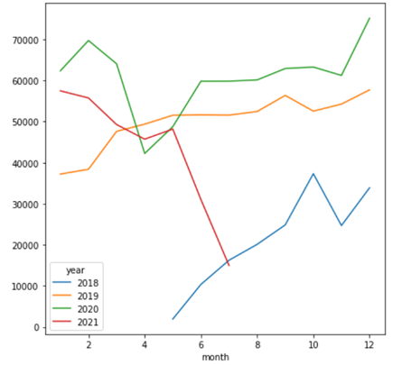
Figure
1 allows the indication of the number of sales per month from 2018 to 2021. By
analyzing the data, we observed that the first year had a lower number of sales
due to the fact that it was an unstable time for the solution with a lower
number of stores. Worth to mention that the second semester has a large number
of sales due to the end of year holiday season. Also, we identify that the
number of sales increased with each year observed, as well as that the highest
occurrence of sales took place on Saturdays and Fridays, while the lowest
number of sales occurred on Sunday. Friday and Saturday are the days that we
identify the highest sales numbers, generally 15% to 20% higher than the other
weekdays. And Sunday is usually 50% higher than Saturday, because many stores
are closed.
Figure 1 - Distribution of sales in each year
Source: The authors.
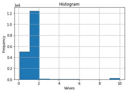
Figure 2 presents a histogram of the analysis about the values of change that
are most frequently purchased according to their price range in Brazilian Real
(BRL).
Another
important measure for analyzing quantitative variables is the scatter plot. By
analyzing the database, it is possible to identify two quantitative measures:
the sales quantity and the sales value. That way, a relationship is created
between the sales price and its respective recurrence. This is important to
identify whether there is a linear relationship between these two variables.
Figure 2 - Histogram of price values
Source: The authors.
The
data analysis identified that the majority of sales are concentrated in values
between R$1 and R$2. It is also possible to conclude that there is a small
recurrence of the values above R$2, appearing to be an almost constant
distribution. Another observation, some outliers that are found in the amount
close to R$10 and R$5. Figure 2 shows the results obtained. Also, it is
possible to conclude that there is a symmetrical distribution of data, with a
small variation in the months of May, June and July. Furthermore, it is
possible to notice that although the prices of the tickets acquired are mostly
between R$1 and R$2, there is a large occurrence of outliers, varying between
R$2 and R$10. This concludes that most outliers are concentrated between R$8
and R$10.
3.3 EXPERIMENTAL METHODOLOGY
The methodology of this
work was carried out according to the steps described below:
·
Step
1:
Selection of models to be used for sales forecasting. Before running the
algorithms, it is necessary to select hyperparameters and also divide the
database.
It is worth mentioning that
initially the holdout method was chosen with the division of training (70%) and
test (30%) mass. However, this method has the disadvantage that the data can be
very biased in the selection of data for training and, therefore, the high
training accuracy does not mean a generalization of learning. And that
generates bad results when the model is used with real data. To solve this
problem, the cross-validation method was used. This method trains and tests the
model with all available data to avoid variance and, thus, ensure more robust
results. The disadvantage of this method is the high computational cost,
however as in this research we have a small database, this was not considered
critical to the point of excluding the use of this method.
·
Step
2:
Represents the choice of metrics for evaluating the performance of the data
obtained. For this, the MSE and the RMSE were chosen. Both are indicated in
problems where predictions that are too far from the real increase the value of
the measure, which makes it an excellent evaluation metric for problems when
large errors are not tolerated, such as in the case of price projections.
Therefore, these two error metrics are described below:
Mean squared error (MSE): The mean squared error is commonly used to
check the accuracy of models and gives greater weight to the biggest errors,
since, when calculated, each error is individually squared and, after that, the
mean of these square errors is calculated.
Root-mean-square error (RMSE): is the measure that calculates "the root
mean square" of errors between observed (actual) values and predictions
(hypotheses) [14].
·
Step
3:
Comparison of techniques for forecasting optimization. In order to analyze the
obtained results, Five algorithms were chosen with two distinct approaches: the
time series prediction and the ensemble method. These techniques were chosen
because they are widely used in various problems and because they are easy to
implement.
·
Step
4:
Hypothesis tests for statistical validation of the results found. In this phase
each method will be compared with the ensemble method to check if there is
improvement of performance or not.
4 RESULTS AND DISCUSSIONS
4.1 RESULTS
To validate the results obtained between all
the analyzed methods the RMSE metric was used as shown in Table 1.
Table 1 - Performance Comparison
|
|
LSTM
|
ARIMA
|
LR
|
SVR
|
RCV
|
ENS.
|
|
RMSE
|
0.99
|
0.104
|
0.131
|
03139
|
0.137
|
0.136
|
Source: The authors.
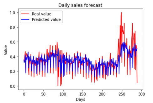
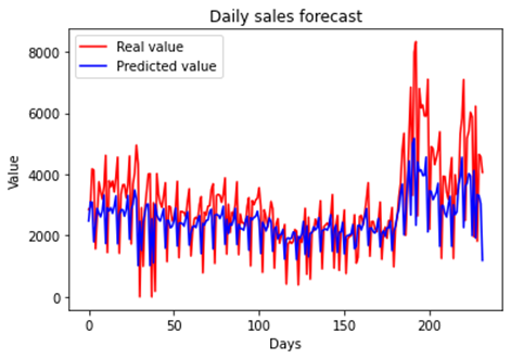
·
LSTM: One of the approaches used for sales forecasting was
the LSTM neural network. This network was implemented using a 4-layer network,
with 50 neurons each, each one with a 20% dropout. As an LSTM, we are
considering the previous 7 days to perform the current forecast. In addition,
the model has a configuration of 150 epochs of the neural network and a batch
size of 32. As a result, Figure 3 shows a graph of LSTM prediction forecast vs
the real.
Figure 3 - LSTM
forecast vs real
Source: The authors.
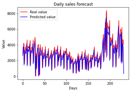
·
ARIMA: The ARIMA model was implemented because it is widely
used in problems with sales forecasting. In the proposed model, the Grid Search
technique was used in order to obtain the best possible parameters for ARIMA.
As a result, it was found that the best combination of hyperparameters was
(6,1,2). In this combination, the model managed to behave well, being able to
predict some peaks. Furthermore, by normalizing the data, an RMSE of 0.1047 was
found, demonstrating a good forecast result as shown in Figure 4.
Figure 4 - ARIMA forecast vs real
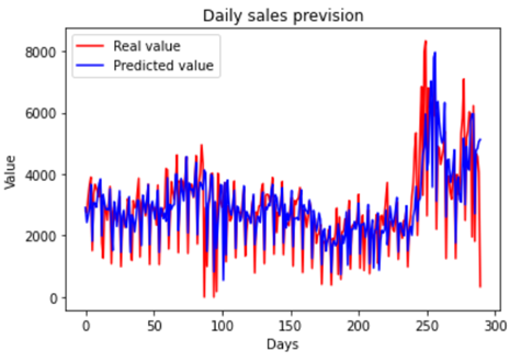
Source: The authors.
·
LR: Linear regression is one of the existing classic models
that was used to forecast sales. For linear regression, a Grid Search was also
implemented, aiming at the optimization of parameters. After that, it was
verified that the parameters that best fit with the LR were: ‘fit_intercept’
false, number of jobs equal to 1, and ‘normalize’ also false. As this is a time
series, to carry out the division between training and database testing, it was
necessary to keep the 'shuffle' parameter (responsible for randomizing the
data) as false. Through this configuration, it was possible to obtain a
reasonable model, but one that cannot predict certain sales peaks. The RMSE can
be found in Table 4 and the result graph in Figure 5.
Figure 5 - LR forecast vs real
Source: The authors.
·
SVR: The SVR technique was also implemented using Grid
Search, to obtain the best possible parameters. In this approach, the ‘shuffle’
parameter also remained false. In addition, the best configuration found was
with the following parameters: 'C' being 10; 'epsilon' being 0.0001; ‘gamma’: 1
and finally, the ‘kernel’ parameter being linear. It was possible to observe
that the model is able to predict behaviors that are repeated and reasonably
predicts some sales peaks as can be noticed in Figure 6. The RMSE of this
technique is shown in Table 4.
Figure 6 - SVR forecast vs real

Source: The authors.
· RIDGE: Another technique that was used was
the Ridge. To obtain the best possible parameters, a Grid Search was also
implemented. From that, the following configuration was obtained: 'alpha' being
0.6; 'fit_intercept' being False and the parameter 'solver' being 'sag'. The
Ridge model was successful in predicting some peaks and dips in sales; in
general, this technique was able to make a good prediction on the behavior of
the time series, as shown in Figure 7. Table 1 also shows the RMSE obtained.
Figure 7 - RCV forecast vs real
Source: The authors.
·
Ensemble
method: The method used was the mean Ensemble
method. That means that the three smaller RMSE algorithms were used as input to
the Ensemble as shown in Table 4. These three techniques were combined to
compose a mean, and this was used as the final result for the combination of
these three algorithms. So, the top
three techniques were: LR (Linear Regression), SVR (Support Vector Machine) and
Ridge, the model was able to reasonably predict the peaks as can be seen in
Figure 8.
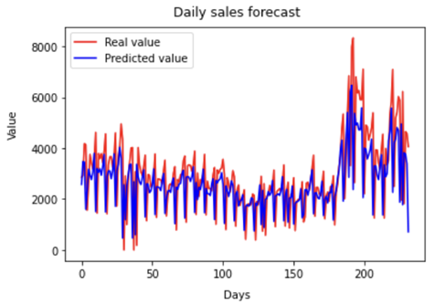
Figure 8 - Ensemble forecast vs real
Source: The authors.
·
Hypothesis
tests: an inquiry method about the veracity of a
statement, associated with maximum risk of error. In other words, by definition
a hypothesis test is a rule decision to accept or reject a hypothesis, based on
the information provided by the data collected in a sample and, therefore,
involves a risk of claiming something wrong [15]. The use of hypothesis tests to assess the
significance of differences between the results of the classical algorithms
before and after the ensemble as a means of determining whether they helped
increase the performance of the prediction algorithm.
After
performing the hypothesis tests comparing the algorithms, it was verified that
the H0 hypothesis was accepted. This means that the result was inconclusive,
that is, there is no statistical evidence with a significance of 5% that there
was an improvement using Ensemble.
4.2 DISCUSSIONS
The work developed in 2013
by Xiaodan, Yu, Zhiquan, Qi, and Yuanmeng, Zhao demonstrates an approach using
Support Vector Regression to forecast magazine sales, in order to avoid
unnecessary prints. In this context, the work used SVR as it states that
multiple and linear regressions can cause overfitting in the model. In fact,
SVR was a good strategy for the problem addressed, as it showed good results.
However, the time series approach has not been developed. Therefore, perhaps
the use of time series models is advantageous for this problem, as applied in
this article, which presented more satisfactory results.
Regarding the work
developed by Passari, it is clear that the intent was to generate models to
forecast sales of individual products. In addition, his research uses
artificial neural networks to detect the relation between variables that impact
product sales, allowing him to make a prediction with greater assertiveness.
Thus, the work proposed here did not use this approach to verifying variables
that may impact sales, which can be considered as a future work using neural
networks to detect possible behaviors related to sales.
On the work done by Zadeh,
Sepehri and Farvaresh, three different approaches were used to predict medical
drug sales. The first approach used an ARIMA model to forecast time series; the
second approach presented a hybrid neural network to forecast the series
through average sales of previous drugs, for each one; the third approach used
a hybrid neural network for time [4]. Through this work, it was possible to see
that the use of hybrid neural networks increases the accuracy of predictions,
as it is able to model non-linear patterns. The present work does not use
hybrid neural networks to model non-linear behaviors, which can be considered a
disadvantage.
5
CONCLUSIONS
With an increasingly
competitive business environment, companies are looking to improve their
operations so that profit is optimized to reduce waste. Companies have invested
in decision support systems to explore scenarios based on the historical data
of their transactions. This way, these systems make it possible to extract
information through large volumes of data to provide insights.
In this work, the ensemble
model was chosen to combine prediction algorithms in order to improve the
performance of predictors. This research presented the proposed ensemble model
that used the averages of the classical algorithms to improve performance, but
this approach did not obtain the expected result. In fact, this approach had
very similar results as classical models independently.
This research shows really
similar results for times series forecasting and ensemble method for optimizing
sales forecasts. Also, it is worth noting that all methods applied in this
research obtained a gain up to 6% of precision compared to the current
technique used by Azure Company for sales forecasting.
As future work, a
comparison with a trainable ensemble model is planned in order to obtain better
results than the proposed approaches in this article. Another possible future
work is the use of neural networks to more accurately obtain non-linear
behaviors and possibly observe the relationship between variables that may
impact sales. Regarding the ARIMA model, a possible improvement of the model
can be done using the SARIMA models, which are useful models for databases with
seasonal behavior. In addition, another important technique will be to train
the database with previous years and predict future years.
REFERÊNCIAS
[1] PASSARI,
A. F. L. Exploração de dados atomizados para previsão de vendas no varejo
utilizando redes neurais. 2003. Tese de Doutorado. Universidade de São
Paulo.
[2] YU, X.; QI, Z.; ZHAO, Y.. Support vector
regression for newspaper/magazine sales forecasting. Procedia Computer
Science, v. 17, p. 1055-1062, 2013.
[3] TRIAYUDI, A. et al. Data mining
implementation to predict sales using time series method. Proceeding of the
Electrical Engineering Computer Science and Informatics, v. 7, n. 2, p.
1-6, 2020.
[4] KHALIL ZADEH, N.; SEPEHRI, M. Mehdi;
FARVARESH, H. Intelligent sales prediction for pharmaceutical distribution
companies: A data mining based approach. Mathematical Problems in
Engineering, v. 2014, 2014.
[5] ENCHEVA, Sylvia et
al. Decision support systems in logistics. In: AIP Conference Proceedings.
American Institute of Physics, 2008. p. 254-256.
[6] CALADO, R. B. Mineração
de Dados Não Estruturados Utilizando uma Combinação de Redes Complexas e
Ensemble Dinâmico. 2019. Dissertação de
Mestrado. Universidade de Pernambuco.
[7] TIAN, Huiren et al. An LSTM neural network for improving
wheat yield estimates by integrating remote sensing data and meteorological
data in the Guanzhong Plain, PR China. Agricultural and Forest Meteorology,
v. 310, p. 108629, 2021.
[8] SWARAJ, Aman et al.
Implementation of stacking based ARIMA model for prediction of Covid-19 cases
in India. Journal of Biomedical Informatics, v. 121, p. 103887, 2021.
[9] VICARI, et al. Modeling of the 2001
lava flow PAVLYSHENKO, Bohdan M. Machine-learning models for sales time
series forecasting. Data, v. 4, n. 1, p. 15, 2019.
[10] PASSARI,
Antonio Fabrizio Lima. Exploração de dados atomizados para previsão de
vendas no varejo utilizando redes neurais. 2003. Tese de Doutorado. Universidade
de São Paulo.
[11] CLEMENTS,
Michael P.; SMITH, Jeremy. The performance of alternative forecasting
methods for SETAR models. International Journal of Forecasting, v. 13,
n. 4, p. 463-475, 1997.
[12] GARDNER JR, Everette S. Exponential
smoothing: The state of the art. Journal of forecasting, v. 4, n. 1, p.
1-28, 1985.
[13] JABBAR, H.; KHAN,
Rafiqul Zaman. Methods to avoid over-fitting and under-fitting in supervised
machine learning (comparative study). Computer Science, Communication and
Instrumentation Devices, p. 163-172, 2015.
[14] CHAI, Tianfeng;
DRAXLER, Roland R. Root mean square error (RMSE) or mean absolute error
(MAE)?–Arguments against avoiding RMSE in the literature. Geoscientific model development, v. 7, n. 3, p.
1247-1250, 2014.
[15] HIRAKATA, Vânia Naomi; MANCUSO, Aline Castello Branco;
CASTRO, Stela Maris de Jezus. Teste de hipóteses: perguntas que você sempre
quis fazer, mas nunca teve coragem. Vol. 39, n. 2, 2019, p. 181-185, 2019.