1 INTRODUCTION

The concept of digital twins is indeed relatively new in its popularized form [1], but its underlying principles have been applied in various industries for many years. Michael Grieves is often credited with introducing the term digital twins in 2002 during a conference in the context of product lifecycle management (PLM). However, it is essential to note that the idea of creating digital representations of physical objects or systems happened before this term was coined.

Historically, there has been little consensus on the exact definition of digital twins, or the terminology used to describe them. This lack of agreement stems from the multidisciplinary nature of digital twins, which can be applied to various of fields, from manufacturing to healthcare, and beyond [2], represented in Figure 1.

Figure 1 – Digital Twins applications

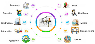
Source: [2]

In 2020, the Digital Twin Consortium was established by member companies to address this problem [3]. The consortium primarily focuses is on standardizing technology and terminology related to digital twins to promote their wider adoption across industries. This effort reflects the growing recognition of the potential benefits that digital twins can offer in terms of improving product design, manufacturing processes, asset management, and overall system performance.

Digital twins create virtual representations of physical objects, systems, or processes to monitor, simulate, and optimize their behavior and performance. These virtual representations are continuously updated with real-time data, allowing for better decision-making, predictive maintenance, and enhanced domain efficiency.

Within the scope of Industry 4.0 and the amount of data provided by the Internet of Things (IoT), it is possible to compute a digital replica of a physical asset. This so-called Digital Twin replica ideally represents all the behaviors and functioning of the physical twin. The high-fidelity Digital Twin model of physical assets can produce system data close to physical reality, which offers extraordinary opportunities for forecasting, simulation, and diagnosis of asset failures. Moreover, in forecasting Digital Twins can be used to optimize the energy consumption of assets, reducing operational costs and environmental impact. They help in fine-tuning parameters for optimal performance while minimizing energy usage.

In this context, this work investigates different forecasting techniques used to build a real-world Industry 4.0 application using concepts of Digital Twins, comparing such methods with real data collected from a temperature sensor during the initial stages of a manufacturing process. As described in Figure 2, sensor data is collected from an industry and its data is consolidated into an IoT Hub to be used as inputs for the different digital twin’s models that are generated from the selected assets of the chosen industry. Finally, this data is presented to the end users as dashboards, graphs, and reports informing them of the real and predicted condition of the equipment.

Figure 2 – Digital Twins applications diagram

A screenshot of a computer

Description automatically generated

Source: Author

The paper is organized as follows. Section 2 outlines the related work on time series forecasting. Section 3 discusses the materials and methods of this article with the results of each selected forecasting method. Section 4 presents a comparison of the results of the selected methods. Section 5 offers the study’s conclusion and list different areas that can be used for future works.

2 BACKGROUND AND RELATED WORKS

2.1 TIME SERIES PREPROCESSING

Univariate time series data, characterized by a sequence of observations recorded at successive time points, find applications in diverse domains, including finance, healthcare, meteorology, and industrial processes. Before employing advanced analysis and forecasting methods, it is crucial to effectively preprocess the data to enhance its quality, remove noise, and ensure reliable results [4], [5], [6].

Outliers, extreme values that deviate significantly from the general trend of the data, can distort statistical analyses and modeling efforts. Techniques such as z-score-based [7] methods can help identify and remove these outliers, ensuring the accuracy of subsequent studies.

IoT-generated time series data can exhibit outliers due to various factors including sensor malfunctions, transient disturbances, or even cyber-attacks. Identifying these outliers is crucial, as they can distort the temporal patterns important to accurate predictions in IoT systems.

The mean absolute deviation (MAD) which its formula is described in equation 1, emerges as a powerful approach to detecting outliers within time series data [7]. Given IoT data’s dynamic and evolution, the MAD method accounts for the absolute deviations of individual data points from the median of the entire time series. This adaptability is particularly valuable in IoT scenarios, where outliers might emerge from previously unseen events or irregularities.

(1)

The values identified as outliers were removed from the time series and the gaps created after the removal were filled using linear interpolation. Missing values are expected in time series data and can arise for various reasons. Imputing missing values is essential to ensure a continuous and complete time series for analysis. Linear interpolation is widely used to estimate missing values based on neighboring observations and is a widely used method [8].

Time series data often vary in scale and magnitude, leading to biased analyses and misleading interpretations. Normalization, whose formula is described in equation 2, ensures that all features are brought to a standard scale, eliminating the dominance of high-scale variables in analyses like clustering, classification, and regression. In the formula, min and max values refer to the normalization of the variable x, and y is the normalized value.

(2)

It is essential to verify the time series stationarity. The Augmented Dickey-Fuller (ADF) [9] test is a widely used statistical test to determine if a time series is stationary [10], meaning that its statistical attributes remain unchanged over the time.

Walk-forward validation using a sliding window [11], represented in Figure 3 and known as rolling validation or moving window validation, is a time series cross-validation technique used to assess the performance of time series forecasting models. Unlike traditional cross-validation, where data is randomly shuffled, maintaining the temporal order of the data, which is crucial for time series analysis, Walk-forward validation simulates the real-world scenario of making sequential predictions as new data becomes available over time.

Figure 3 – Walk Forward validation with a sliding window.

A screenshot of a graph

Description automatically generated

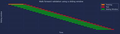
Source: Author.

Walk-forward validation also considers the model to be fitted every time the window is moved forward along the time series. Still, since the collected data from the sensor is a stationary time-series, it is not necessary to re-fit the model. This represents less computational requirements during the execution of tests and during the usage of the model in real-time with new data from the sensors.

A primary advantage of this method is that more data is used to train and test the model without having to use a validation set and without the risk of overfitting [12].

2.2 FORECASTING METHODS

2.2.1 Baseline methods

As baseline methods, we considered the Naïve and Naive Drift approaches. Both serve as reference points for evaluating the performance of more complex forecasting models. These methods provide simple and straightforward predictions that can be used to benchmark the effectiveness of more sophisticated techniques.

The Naive method predicts that the next value will be the same as the last observed value using the formula described in eq. 3 It assumes that there is no change or trend in the data. The equation uses the value for using the previous value of the time series.

(3)

Naive Drift, or the Drift method, is a basic forecasting technique that assumes a linear trend in the time series data. It is an extension of the Naive method, which predicts that the next value will be the same as the last observed value. The Naive Drift method, however, considers the time elapsed between observations and adjusts the prediction based on this elapsed time, effectively incorporating a linear trend or drift into the forecast.

2.2.2 Statistical methods

Statistical forecasting uses historical data and statistical techniques to predict time series values and other data types.

The ARIMA (Auto Regressive Integrated Moving Average) method was developed and introduced in the early 1970s [13]. The fundamental concepts behind ARIMA were established by the statisticians George E. P. Box and Gwilym M. Jenkins, and their work is documented in the book titled ”Time Series Analysis: Forecasting and Control”, which was first published in 1970. This method is still being used for time series forecasting due to its good results, including forecasting using industrial sensor data [14] [15] [16]. Another advantage of this method is that it when only has limited historical data from the sensors to use during the training phase [17].

2.2.3 Machine Learning

Machine learning can be used for univariate time series forecasting by leveraging patterns and relationships within historical data to predict future values of a single variable over time.

Recurrent Neural Networks (RNNs) are artificial neural network architecture that handle sequence data, such as time series. Unlike traditional neural networks that process each input individually, RNNs have feedback connections, allowing previous information to influence the processing of subsequent inputs. The critical feature of RNNs is their ability to maintain an internal memory or hidden state, which is updated with each new input and influences future processing. This memory enables RNNs to capture long-term dependencies in data sequences, making them particularly useful in situations when the previous context is relevant for understanding the current context.

In the paper [18], Hochreiter and Schmidhuber proposed the LSTM architecture to solve the vanishing gradient problem that can occur in traditional recurrent neural networks (RNNs). The key element that gives the capability to capture long-term dependencies to LSTM is called memory block and described in Figure 4.

Figure 4 – LSTM diagram

Sem título.png

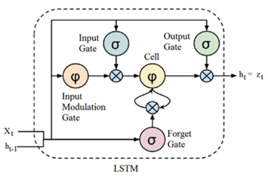
Source: [19].

Due to this memory block, LSTMs can handle long-range dependencies and capture patterns in sequences over extended time intervals, making them highly suitable for tasks involving sequential data, such as time-series forecasting [19] [20] [21] [22].

2.4 HYPERPARAMETERS SEARCH

Hyperparameter search is the process of finding the best set of hyperparameters for a machine learning model [23]. Hyperparameters are parameters that control the learning process of the model but are not learned from the data. Some common examples of hyperparameters include the learning rate, the number of epochs, and the number of hidden layers in a neural network.

2.5 FORECASTING ACCURACY

Forecasting accuracy refers to the degree of closeness between the predicted values from a forecasting model and the real data of the target variable. It measures how well a forecasting model can accurately capture the underlying patterns, trends, and variations in the data to make accurate predictions of future values.

The forecast accuracy measures are always calculated using test data that were not used when computing the forecasts [24]. When using forecasts that are on the same scale, the root mean square error (RMSE) is one of the recommended methods and it is defined using the formula in (4). In the equation n is the number of observations, is the real observed value at time, and is the predicted value at time .

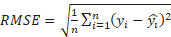(4)

3 MATERIALS AND METHODS

This section provides a comprehensive overview of the executed steps. It begins with data loading, followed by preprocessing. Next, we delve into training using four distinct methods. Finally, we present the results obtained from these methods.

3.1 DATA SET

The first step executed during this study was to perform the data preprocessing required on the collected data from the industrial sensors. The collected sensor data was saved in a CSV file, including the timestamp and temperature attributes. The dataset range starts from 00:00 of 1^st of June of 2022, to 23:59 of June 29, 2022 with a total of 88,741 sensor readings. This represents an average of 3,060 readings per day.

The data from this CSV was loaded as a time series and plotted using a Python data visualization library called Matplotlib [26] to execute the first visual inspection and analysis. During this first visual inspection of Figure 6, it was possible to see a similar behavior of the time series along the collected period, indicating the time series could be identified as stationary and requiring a stationarity test to be executed [9].

3.2 PREPROCESSING

The subsequent step involved identifying outliers using mean absolute deviation (MAD), eliminating them, and then employing linear interpolation to fill the gaps left in the time series due to these removals. This process detected and replaced 1,031 outliers in the time series and can be visualized in Figure 7. The total length of the time series was not affected because all removed outliers were replaced using linear interpolation.

Another executed step was to verify the time series stationarity to validate this hypothesis identified in the visual inspection after plotting the time series. The Augmented Dickey–Fuller (ADF) [9] test was executed and confirmed the collected sensor data created a stationary time series. The ADF test returned a p-value equals to 3.408511793361129e−29, and since this value is less than or equal to 0.05, H0 was rejected, and stationarity was confirmed.

The data set was then split into training and test data sets. The division of 80/20 was used to split, meaning the training data set was created with 80% of the values total and test 20%. Their sizes were 70,992 and 17,749 sensor readings. After this split, both data sets were normalized as described in section 2.1 using the normalization parameters obtained from the training data set. The result of this step can be observed in Figure 8.

3.3 EXPERIMENTAL METHODOLOGY

The forecast range selected in our experiments was from one step forward to ten steps. The forecasting used walk-forward validation with a sliding window described in Figure 3. The sliding window size was set according to the forecasting range for each iteration of the test. This means the executed test was repeated 10 times with different forecasting ranges, varying from 1 to 10.

The first baseline forecasting method executed was the Naive forecast. The forecast horizon selected for this method was from one step to ten steps forward. The forecast was executed using the test data set for each different value of the forecast horizon and always using the previous observed value to determine the forecasted values. The accuracy of this method is presented in Table 1.

Table 1 – Naive Forecasting RMSE.

Forecast horizon	RMSE
1 step	0.020107
2 steps	0.028467
3 steps	0.035618
4 steps	0.040981
5 steps	0.047885
6 steps	0.053208
7 steps	0.054365
8 steps	0.059190
9 steps	0.064050
10 steps	0.069753

Source: Author.

The following executed forecasting method was Naive Drift and the same forecasting horizons from the previous method were also used in this one as well. For this method, different subsets of the training data set were used to verify if smaller training subsets can speed up the training phase without compromising the accuracy of the forecasts. The training data sets were tested using the lengths described in Table 2.

Table 2 – Training data set lengths used for in models.

Training data set lengths
50
100
500
1000
10,000
20,000
50,000
70,000

Source: Author.

After some preliminary experiments, the best accuracy with the lower RMSE was observed with 50,000 values from the training data set. Using the complete data set or more significant amounts was unnecessary to achieve better accuracy for this forecasting method. The result of this method was very similar when compared to the previous method, Naive, even having much more data being used for the training compared to Naive since it only uses the previous n readings. One of the possible reasons for this is due to the high-frequency nature of the time series used in this experiment, which helps in the first method. The RMSE for this method is described in Table 3.

Table 3 – Naive Drift Forecasting lowest RMSEs.

Forecast horizon	RMSE
1 step	0.020107
2 steps	0.028467
3 steps	0.035619
4 steps	0.040982
5 steps	0.047886
6 steps	0.053210
7 steps	0.054367
8 steps	0.059192
9 steps	0.064053
10 steps	0.069757

Source: Author.

Auto ARIMA was also executed with the same data set and the same forecasting horizons as the previous method. The length of the training data set was also tested using the different values defined in Table 2, using the same approach as the Naive Drift method that was previously executed. As was initially expected, this method resulted in better accuracy than the baseline methods. Moreover, according to Table 7 some scenarios of multistep ahead required less training to obtain better accuracy. The RMSE of this method is described in Table 4 and Table 7, the latter includes the length of the training data set that resulted in the lowest RMSE value. For this method, the StatsForecast [26] Python library was used.

Table 4 – Auto ARIMA Forecasting lowest RMSEs.

Forecast Horizon	RMSE
1 step	0.018433
2 steps	0.026235
3 steps	0.033717
4 steps	0.039248
5 steps	0.043817
6 steps	0.051401
7 steps	0.052531
8 steps	0.055412
9 steps	0.064519
10 steps	0.066474

Source: Author.

After completing the tests with the baselines and statistical methods, the same data set was executed using a Long Short-Term Memory (LSTM) recurrent neural network [18]. This model was selected because of its ability to capture long-range dependencies [18] and due to this it can effectively handle sequential data such as time-series, which is the case in the dataset being used in this study.

The first executed step was the hyperparameters tuning. This was done using an open-source Python package for hyperparameter optimization framework named Optuna [23] that allows to dynamically define the hyperparameters search space to find its optimal values. The hyperparameters search was executed using the following ranges.

· Number of layers: 1 - 100

· Size of hidden layer: 1 - 250

· Dropout: 0.0 – 0.9

· Epochs: 1 - 999

As a result of this search, the following values were found and used in the LSTM model:

· Number of layers: 1

· Size of hidden layer: 11

· Dropout: 0.12491736459588197

· Epochs: 405

· Learning Rate: 1e-3

· Optimizer Class: Adam

The RMSE obtained by this method can be visualized in Table 5.

Table 5 – LSTM Forecasting lowest RMSEs.

Forecasting Horizon	RMSE
1 step	0.016199
2 steps	0.020448
3 steps	0.025473
4 steps	0.028625
5 steps	0.031311
6 steps	0.035913
7 steps	0.036612
8 steps	0.038325
9 steps	0.044608
10 steps	0.044678

Source: Author.

4 RESULTS COMPARISON

The first step was to verify with the Friedman test [28] if there is significant statistical difference observed across the collected values or if they could have occurred by chance. The test returned p-value rejecting the null hypothesis of the test, meaning there are significant differences among the obtained RMSEs from each method.

Then, a comparison between the selected methods using the lowest RMSE values collected for each forecast horizon regardless of the length of the training data set, which means that the optimal size of the training data set was used in this first comparison. As presented in Table 6, LSTM outperformed the other methods in all different forecasting horizon scenarios. Auto ARIMA was the second on the list followed by Naive Drift and Naïve, which obtained similar values for the RMSE. LSTM outperformed Auto ARIMA by an average of 4.83%. Auto ARIMA outperformed Naive Drift and Naive by an average of 21.30%.

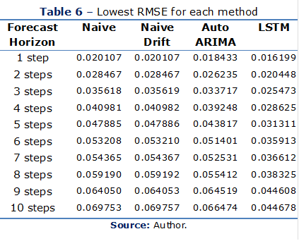
Figure 9 and 10 shows the comparison among all selected methods to their forecasting time. The first image presents the amount of time that each method took to execute the forecasting for all horizons. The second image presents the average time for each forecasting step, also in horizons.

It was also observed in Figure 11 that LSTM underperforms statistical methods when using small training data sets. The same figure shows that the LSTM outperforms the other selected methods only when the training data set contains at least 500 sensor readings.

5 CONCLUSIONS

In this work, we present different forecasting techniques used to build a real-world Industry 4.0 application using concepts of Digital Twins. This experiment used real data collected from a temperature sensor during the initial stages of a manufacturing process were used.

The provided results contain information to conclude that LSTM obtained a better outcome for the RMSE when using large training data sets. LSTM got similar or lower results when working with a small training data set. This means that LSTM must be carefully selected depending on the amount of data available to train the model. Moreover, Figure 9 and 10 shows LSTM taking more processing time than the other selected methods in the forecasting phase. It also adds an extra step in the process: which is the hyperparameters search before fitting the model.

It is also clear that, despite the discussed drawbacks of using LSTM models, its accuracy gains can have a significant positive impact, especially in the context of Digital Twins and industrial applications [29]. The following points can be observed:

· Accuracy Gains: LSTM models are known for capturing sequential patterns and dependencies in data, making them valuable for time series forecasting and predictive modeling. Given that it resulted in improved accuracy, it can lead to more reliable predictions and decision-making. According to

the results presented in this work, LSTM outperformed Auto ARIMA by an average of 4.83%, which be enough to avoid equipment faults and reduced maintenance tasks.

· Reduced Resource Usage: By achieving more accurate predictions, the usage of industrial, such as natural gas and electricity, can be optimized. This means that utility resources can be used more efficiently, potentially reducing costs, minimizing waste, and reducing the environmental impact.

· Financial Impact: Even small gains in RMSE can translate to significant cost savings in an industrial environment. This is particularly crucial in industries where energy consumption, resource utilization, and operational efficiency are closely monitored and directly impact on the bottom line.

In summary, despite the potential drawbacks of using LSTM models, their ability to enhance accuracy and, consequently, reduce resource consumption and costs can make them a valuable tool in the context of Digital Twins and industrial operations. However, it's important to continue refining and fine-tuning these models to mitigate their limitations and maximize their benefits.

The following topics can be used for future work around the subject of this paper.

· How to identify the most optimal length of the training data set without having to test different lengths?

· Execute comparisons using different multi-step ahead forecast strategies, such as recursive, direct and hybrid.

· Execute forecasting using multivariate timeseries by using information from other digital twin’s sensor data and its geolocations. With the objective to predict failures and reduce utility consumption.

REFERENCES

[1] GRIEVES, Michael; VICKERS, John. Origins of the digital twin concept. Florida Institute of Technology, v. 8, p. 3-20, 2016.

[2] ATTARAN, Mohsen; CELIK, Bilge Gokhan. Digital Twin: Benefits, use cases, challenges, and opportunities. Decision Analytics Journal, p. 100165, 2023.

[3] OLCOTT, S.; MULLEN, C. Digital twin consortium defines digital twin. Available at: blog.digitaltwinconsortium.org/2020/12/ digital-twin-consortium-defines-digital-twin.html, 2020.

[4] BLÁZQUEZ-GARCÍA, Ane et al. A review on outlier/anomaly detection in time series data. ACM Computing Surveys (CSUR), v. 54, n. 3, p. 1-33, 2021.

[5] KHAYATI, Mourad et al. Mind the gap: an experimental evaluation of imputation of missing values techniques in time series. In: Proceedings of the VLDB Endowment. 2020. p. 768-782.

[6] LIMA, Felipe Tomazelli; SOUZA, Vinicius MA. A Large Comparison of Normalization Methods on Time Series. Big Data Research, v. 34, p. 100407, 2023.

[7] LEYS, Christophe et al. Detecting outliers: Do not use standard deviation around the mean, use absolute deviation around the median. Journal of experimental social psychology, v. 49, n. 4, p. 764-766, 2013.

[8] TROYANSKAYA, Olga et al. Missing value estimation methods for DNA microarrays. Bioinformatics, v. 17, n. 6, p. 520-525, 2001.

[9] MUSHTAQ, Rizwan. Augmented dickey fuller test. 2011.

[10] FULLER, Wayne A. Introduction to statistical time series. John Wiley & Sons, 2009.

[11] VAFAEIPOUR, Majid et al. Application of sliding window technique for prediction of wind velocity time series. International Journal of Energy and Environmental Engineering, v. 5, p. 1-7, 2014.

[12] BERGMEIR, Christoph; BENÍTEZ, José M. On the use of cross-validation for time series predictor evaluation. Information Sciences, v. 191, p. 192-213, 2012.

[13] BOX, G.E.P.; JENKINS, G. M.; REINSEL, G. C. Time series analysis: forecasting and control. John Wiley & Sons, 2011.

[14] KANAWADAY, A.; SANE, A. Machine learning for predictive maintenance of industrial machines using IoT sensor data. In: 2017 8th IEEE international conference on software engineering and service science (ICSESS). IEEE, 2017. p. 87-90.

[15] ZHANG, Weishan et al. LSTM-based analysis of industrial IoT equipment. IEEE Access, v. 6, p. 23551-23560, 2018.

[16] MANI, Geetha; VOLETY, Rohit. A comparative analysis of LSTM and ARIMA for enhanced real-time air pollutant levels forecasting using sensor fusion with ground station data. Cogent Engineering, v. 8, n. 1, p. 1936886, 2021.

[17] ELSARAITI, Meftah; MERABET, Adel; AL-DURRA, Ahmed. Time Series Analysis and Forecasting of Wind Speed Data. In: 2019 IEEE Industry Applications Society Annual Meeting. IEEE, 2019. p. 1-5.

[18] HOCHREITER, Sepp; SCHMIDHUBER, Jürgen. Long short-term memory. Neural computation, v. 9, n. 8, p. 1735-1780, 1997.

[19] CHHAJER, Parshv; SHAH, Manan; KSHIRSAGAR, Ameya. The applications of artificial neural networks, support vector machines, and long–short term memory for stock market prediction. Decision Analytics Journal, v. 2, p. 100015, 2022.

[20] TAN, Mao et al. Ultra-short-term industrial power demand forecasting using LSTM based hybrid ensemble learning. IEEE transactions on power systems, v. 35, n. 4, p. 2937-2948, 2019.

[21] ZHANG, Weishan et al. LSTM-based analysis of industrial IoT equipment. IEEE Access, v. 6, p. 23551-23560, 2018.

[22] COOK, Andrew A.; MISIRLI, Göksel; FAN, Zhong. Anomaly detection for IoT time-series data: A survey. IEEE Internet of Things Journal, v. 7, n. 7, p. 6481-6494, 2019.

[23] AKIBA, Takuya et al. Optuna: A next-generation hyperparameter optimization framework. In: Proceedings of the 25th ACM SIGKDD international conference on knowledge discovery & data mining. 2019. p. 2623-2631.

[24] HYNDMAN, Rob J. Measuring forecast accuracy. Business forecasting: Practical problems and solutions, p. 177-183, 2014.

[25] HYNDMAN, Rob J.; KOEHLER, Anne B. Another look at measures of forecast accuracy. International journal of forecasting, v. 22, n. 4, p. 679-688, 2006.

[26] HUNTER, John D. Matplotlib: A 2D graphics environment. Computing in science & engineering, v. 9, n. 03, p. 90-95, 2007.

[27] GARZA, Federico et al. StatsForecast: Lightning fast forecasting with statistical and econometric models. PyCon: Salt Lake City, UT, USA, 2022.

[28] FRIEDMAN, Milton. A comparison of alternative tests of significance for the problem of m rankings. The annals of mathematical statistics, v. 11, n. 1, p. 86-92, 1940.

[29] CHOI, Eunjeong; CHO, Soohwan; KIM, Dong Keun. Power demand forecasting using long short-term memory (LSTM) deep-learning model for monitoring energy sustainability. Sustainability, v. 12, n. 3, p. 1109, 2020.

A Comparative Study of Forecasting Methods in the Context of Digital Twins

1 INTRODUCTION

2 BACKGROUND AND RELATED WORKS

A Comparative Study of Forecasting Methods in the
Context of Digital Twins